This is a comprehensive manual for the graphical interface to StatAlign. Command-line-specific information can be obtained by running
java -jar StatAlign.jar -helpThe documentation on this page can be navigated by using the hyperlinks and the Forward and Backward buttons of your browser. This manual can also be accessed from within StatAlign, via the Help → User's manual menu. When using the latter method, clicking the Home button reloads this page.
StatAlign provides a unified approach for inferring multiple
sequence alignments, evolutionary trees and model parameters within a joint Bayesian framework.
Most other methods for phylogenetic inference use a single fixed alignment as input. However, this
can result in significant bias in the resulting trees, since the results may be very sensitive to
the specific choice of alignment. In addition, these methods typically treat
insertions and deletions (gaps) as missing data, discarding a great deal of important information
in the process, and potentially further biasing the results.
To address these problems, StatAlign jointly samples multiple alignments, evolutionary trees
and model parameters under a stochastic model of substitution, insertion and deletion
![]() , making use of a Markov chain Monte Carlo scheme
, making use of a Markov chain Monte Carlo scheme
![]() to generate samples from the desired posterior distribution.
The program allows a range of different substitution models; the insertion-deletion model
is a modification of the TKF92 model
to generate samples from the desired posterior distribution.
The program allows a range of different substitution models; the insertion-deletion model
is a modification of the TKF92 model
![]() , which allows 'refragmentation' at internal nodes. For more details,
see Miklós et al. (2008)
, which allows 'refragmentation' at internal nodes. For more details,
see Miklós et al. (2008)
![]() .
.
Users can load sequences, and choose a substitution model with which to analyze
the sequences. Once the parameters of the Markov chain and desired output are specified
(e.g. log-likelihood trace, alignment, tree samples etc.), the MCMC chain can be initialised,
generating a set of samples for the parameters of interest, as well as
consensus alignments and trees.
The following sections contain descriptions of the graphical elements of the program (menu bar,
tabulated panels, pop-up dialog windows), with examples illustrating how an analysis can be carried
out.
In the File menu, we can load sequences (and other types of data if supported by plugins), set the output preferences and exit the program.
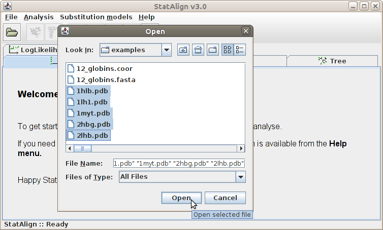
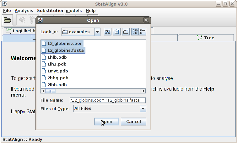
Clicking this menu item will result the pop up of a file opening dialog window.
We can browse the directories in this window and open a file. The file to be opened
should contain sequences in Fasta file
![]() format (and potentially other types of data, when appropriate plugins exist).
Sequences can be viewed and removed via the
Sequences panel.
format (and potentially other types of data, when appropriate plugins exist).
Sequences can be viewed and removed via the
Sequences panel.
Clicking this menu item will pop up a dialog window where you can set up your output preferences
Exits StatAlign.
[ The menu bar ]After loading your sequences and choosing your Model and Output settings, you can click this menu item to set the MCMC parameters and start the MCMC analysis.
Information will be given about the progress of the MCMC sampling in the Status bar, such as the number of burn-in steps completed and the number of MCMC samples taken. The Postprocessing panels will show both snapshots from the MCMC chain, as well as various summaries calculated from the MCMC samples.
We can pause an active MCMC run by clicking this button.
A suspended run can be continued by clicking here.
This item stops an MCMC run. Output files will still be created from the samples that have been taken so far, but you won't be able to restart the process from the same point. This should be used only if you indeed want to terminate the MCMC run early.
[ The menu bar ]
This menu is for selecting the substitution model that is used for analyzing the sequences.
StatAlign automatically recognises the sequences, and if sequences cannot be
analysed by the chosen model (for example, protein sequences are forced to be
analysed by a nucleotide model), a pop-up error box notifies the user.
Implemented models are:
When StatAlign completes a run, it outputs files containing the results of the MCMC sampling. By default, the alignment and total log-likelihood for each MCMC sample are written to a .log file, which also contains a report of the acceptance rates for each MCMC move.
Additional MCMC output is generated by postprocessing plugins, which extract properties of interest from each MCMC sample. This output can either be added to the .log file, or sent to individual files.
The table below shows the default set of output files generated:
| File extension | Contents |
| .tree | Sampled trees (Nexus format) |
| .ctree | Consensus tree taken from samples so far. Internal nodes are labelled with posterior probability for the split preceding the node. |
| .coreModel.params | Parameters of the core evolutionary model (usually indel and substitution rates) |
| .ll | Log likelihood for each MCMC sample. The first column contains the contribution from the core evolutionary model, and the second column contains the total including contributions from model extension plugins. |
| .mpd.ali | Contains the minimum-risk (also termed maximum posterior decoding) summary alignment. |
| .mpd.scores | Per-column marginal posterior probabilities for each alignment column in the MPD alignment. |
| .ali | Sampled alignments (several possible formats). By default this file is not created, since the alignments are printed to the .log file instead. |
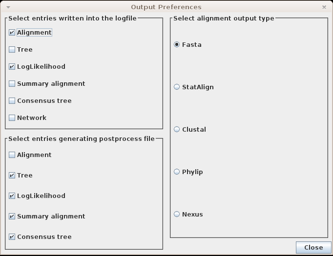
Below we describe the possible settings in this window.
On the top left corner of the output preferences window, users can choose which postprocesses write into the logfile. The format of the output is the following:
Sample [sample_number] [TAB] postprocess_name: [TAB] data
For example, selecting to output just the tree and log-likelihood to the log file, we will obtain a file containing the following:
		Sample 0        Loglikelihood:  -3718.11540541795
		Sample 0        Tree:   ((P1_1aeia:0.05535,((P1_1ann:0.10414,P1_1axn:0.04547):0.01,(P1_1ala:0.02321,P1_1avha:0.01238):0.07713):0.01):0.03021,P1_2ran:0.08613);
		Sample 1        Loglikelihood:  -3620.5414903951587
		Sample 1        Tree:   ((P1_1aeia:0.05535,((P1_1ann:0.10414,P1_1axn:0.04547):0.01,(P1_1ala:0.02321,P1_1avha:0.07235):0.07713):0.01):0.03021,P1_2ran:0.12924);
		Sample 2        Loglikelihood:  -3618.189925496592
		Sample 2        Tree:   ((P1_1aeia:0.05535,((P1_1ann:0.10414,P1_1axn:0.04547):0.01,(P1_1ala:0.02321,P1_1avha:0.11236):0.07713):0.01):0.04352,P1_2ran:0.11424);
		Sample 3        Loglikelihood:  -3615.7331381880526
		Sample 3        Tree:   ((P1_1aeia:0.05535,((P1_1ann:0.10414,P1_1axn:0.04547):0.01,(P1_1ala:0.02321,P1_1avha:0.11236):0.07713):0.01837):0.04352,P1_2ran:0.11424);
		Sample 4        Loglikelihood:  -3587.894867267956
		Sample 4        Tree:   ((P1_1aeia:0.05535,((P1_1ann:0.10414,P1_1axn:0.06347):0.01,(P1_1ala:0.02321,P1_1avha:0.11236):0.07713):0.01837):0.04352,P1_2ran:0.11424);
		Sample 5        Loglikelihood:  -3585.9665576563943
		Sample 5        Tree:   ((P1_1aeia:0.05535,((P1_1ann:0.10414,P1_1axn:0.06347):0.01,(P1_1ala:0.02321,P1_1avha:0.11236):0.08542):0.01837):0.04352,P1_2ran:0.11902);
		Sample 6        Loglikelihood:  -3551.4723341911595
		Sample 6        Tree:   ((P1_1aeia:0.05535,((P1_1ann:0.10414,P1_1axn:0.06347):0.05301,(P1_1ala:0.02321,P1_1avha:0.11236):0.08542):0.03414):0.04352,P1_2ran:0.11902);
			.
			.
			.
[ Output preferences ]
As discussed above, users also can choose which postprocesses generate their own output file. This file has its own format, and may be different from the format written to the log file. For example, the tree postprocess writes the sampled trees into a standard Nexus file
![]() as its own output file. Model extension plugins may also generate their own output files, and when the extension is selected and activated, the corresponding output options will be visible in the Output preferences dialogue box.
as its own output file. Model extension plugins may also generate their own output files, and when the extension is selected and activated, the corresponding output options will be visible in the Output preferences dialogue box.
Supported alignment formats are:
It prints both the sequences at the leaves and the sequences predicted for the internal nodes. The sequence names and the alignment is separated by a TAB. The predicted sequences for the internal nodes contains and empty record for their name. Each sequence in the alignment is shown in one line.
The first line contains the word "Clustal".
The alignment is broken into 60 character wide blocks.
The sequence names are shown at the begining of the line.
Alignment columns with all matches are marked with an
asteriks. See also
![]()
Alignment names are marked with a ">" symbol
and are in a separated line. Alignments are broken into
60 character wide blocks. Each sequence are printed separately, so
it is not easy to see which character is aligned to which one.
See also
![]()
The first line contains the number of sequences and the
length of the alignment. The alignment is broken into 60
character wide blocks, and a space is inserted after each 10 character long
part. The name of the sequences are shown at the begining of the
first block. See also
![]()
Nexus has its own XML-like format. A nexus alignment contains
a header containing information about the seuqence type, sequence names, etc.
See also
![]()
The MCMC parameters dialog window can now be opened by clicking on the tool icon
![]() , which opens up the MCMC settings dialogue panel.
, which opens up the MCMC settings dialogue panel.
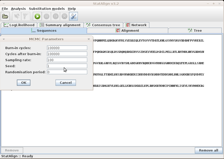
The Markov chain underlying the MCMC simulation takes a certain amount of time to converge to its equilibrium distribution. Only when this convergence is complete will the samples be generated from the correct posterior distribution that we are interested in. This convergence period is called burn-in phase. Users can set how many steps at the beginning of the Markov chain should be treated as the burn-in period. The number of steps necessary for convergence may vary significantly for different datasets, and it is important to check that the chain has successfully converged.
This is the number of Markov chain steps to be taken after the burn-in phase. During these steps, the samples are assumed to be from the desired posterior distribution, and are used for inference.
After each c steps during the post burnin-in period, the state of the Markov chain is recorded, and postprocessed.
The Java language provides a random number generator that generates the
pseudo-random numbers
![]() based on a so-called seed. Users can set this seed here.
The program generates the same result when the same seed is used.
This is useful when one wants to reproduce the result of a run.
In order to check convergence of the Markov chain, the analysis
should be repeated with the same dataset using different random
seeds, to generate multiple independent runs.
based on a so-called seed. Users can set this seed here.
The program generates the same result when the same seed is used.
This is useful when one wants to reproduce the result of a run.
In order to check convergence of the Markov chain, the analysis
should be repeated with the same dataset using different random
seeds, to generate multiple independent runs.
This specifies the length of period at the start of the MCMC simulation during which the state of the chain should be randomly perturbed by accepting all proposed moves. The purpose of this is to test the sensitivity of the final results to the initial conditions. The main randomisation occuring in this period is for the tree topology, since most other parameters typically lose memory of their initial state very quickly. A randomisation period of a few hundred steps combined with different random seeds is typically sufficient to ensure that multiple MCMC runs start from significantly different configurations.
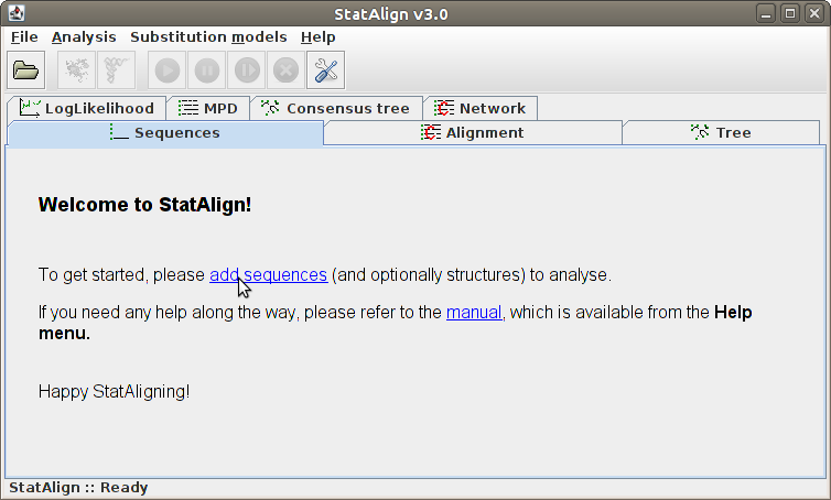
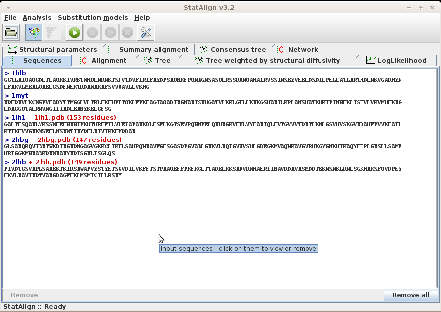
Sequences can be loaded from the menu, following File → Add sequence(s)..., or by selecting the link in the welcome page.
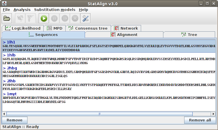
To remove a sequence from the list, click into the desired sequence and
then to the Remove button. Adding sequences can be done simply
by following File → Add sequence(s)....
The sequences are automatically recognised if they are nucleotide or
protein sequences, and a default substitution model is associated to them.
If the sequences are not recognised, an error message is shown, indicating
what are the unknown characters in the input sequences.
When other types of data are added and associated with each sequence, for example
protein structures, these will also appear
alongside the sequence name.
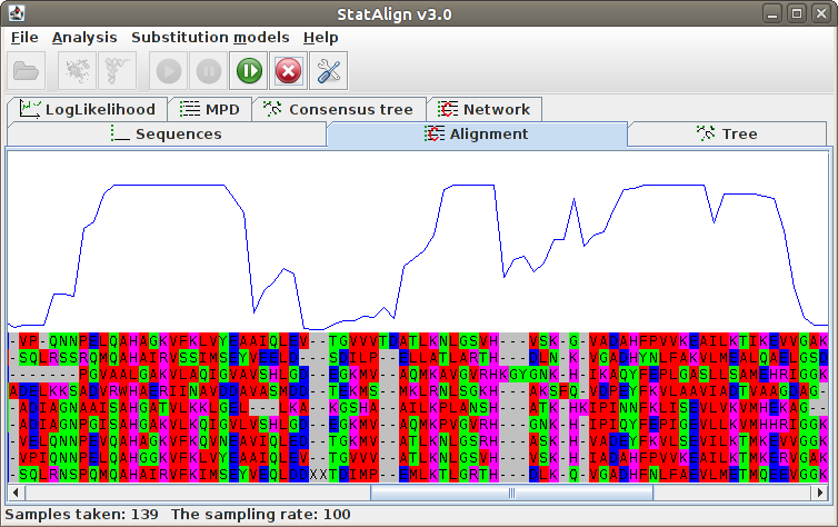
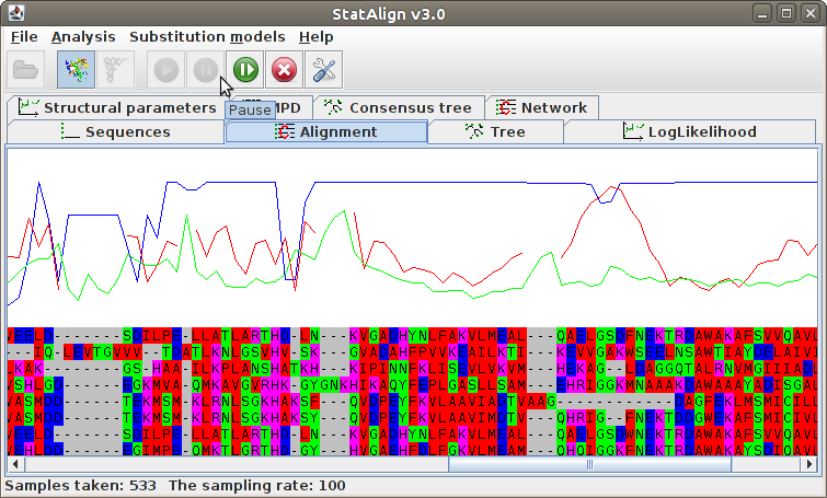
The MCMC algorithm takes a random walk on the joint distribution of alignments, trees and evolutionary parameters. The current alignment can be seen on the Alignment panel. Above the alignment is shown the posterior probability of each alignment column, as estimated from the samples taken so far. This is shown in blue once the burn-in period is over.
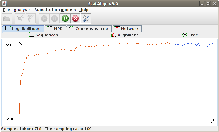
The log-likelihood trace is printed onto the screen, to assist with assessing convergence of the chain. The burn-in phase is coloured in red, and the post burnin-in phase in blue:
The program estimates summarises the alignment samples so far to produce a
type of consensus alignment, using maximum posterior decoding (MPD)
![]() .
The posterior probabilities for each column are printed on top of the alignment, indicating
the reliability of the corresponding MPD alignment column.
.
The posterior probabilities for each column are printed on top of the alignment, indicating
the reliability of the corresponding MPD alignment column.
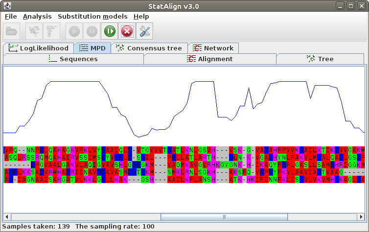
The MPD alignment is estimated using only alignment samples from the after-burn-in period, hence the alignment is not shown during the burn-in phase in this panel.
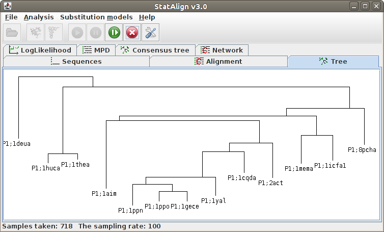
[ The Post-processing tabulated panels ]This panel shows the current tree in the Markov chain.
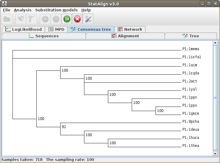
This panel shows the majority consensus tree constructed from all the tree samples taken so far
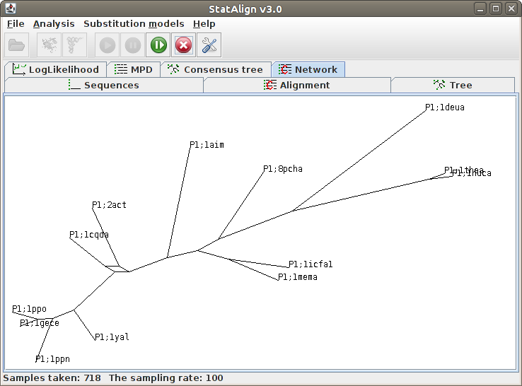
This is similar to the consensus tree, except that unresolved splits are shown as cycles in a graph, indicating all sampled relationships.
java -jar StatAlign.jar -help:structal
>name1
36.587	49.012	31.672	 54.01
35.023	49.494	28.184	 53.01
...     ...     ...      ...
>name2
58.559	46.653	71.532	 62.34
57.828	45.597	67.975	 55.06
...     ...     ...      ...
The first three columns represent the x, y and z coordinates of a single atom associated with each residue in the structure. Typically this will be the alpha carbon. The name of the structure should appear before the start of the coordinates, and the names (name1 and name2 in the above example) should match the names of the sequences to which the structures will be associated. The fourth column is optional, and contains the crystallographic B-factors associated with each triplet of atomic coordinates. If present, the B-factor data is used to allow structural heterogeneity to be incorporated into the evolutionary model. (This information is included by default when structures are read in from a PDB file.)
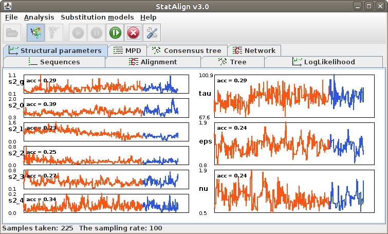
| Parameter name | Meaning |
| τ | Overall structural variance (similar to squared radius of gyration, units of Å2) |
| ε | Amount of structural variability attributed to background (non-evolutionary) fluctuations |
| σ2g | Global structural diffusivity (Å2 / subst. per site) |
| σ2k | Branch-specific structural diffusivity (Å2 / subst. per site) |
| ν | Variance of branch-specific diffusivity parameters (on a log scale) |
The RNA plugin performs secondary structure predictions from multiple alignment samples generated by StatAlign. Both a SCFG approach (PPfold)
and a thermodynamic (RNAalifold) are available.
The advantage of this method of secondary structure prediction is that it considers multipled sampled alignments instead of just a single fixed alignment, as is typically the
case with comparative secondary structure prediction.
Here we describe the options available through the graphical interface.
Options available through the command line interface can be listed by running
java -jar StatAlign.jar -help:rnaalifold
java -jar StatAlign.jar -help:ppfoldThe following flowchart summarises what StatAlign does when RNA mode is enabled:
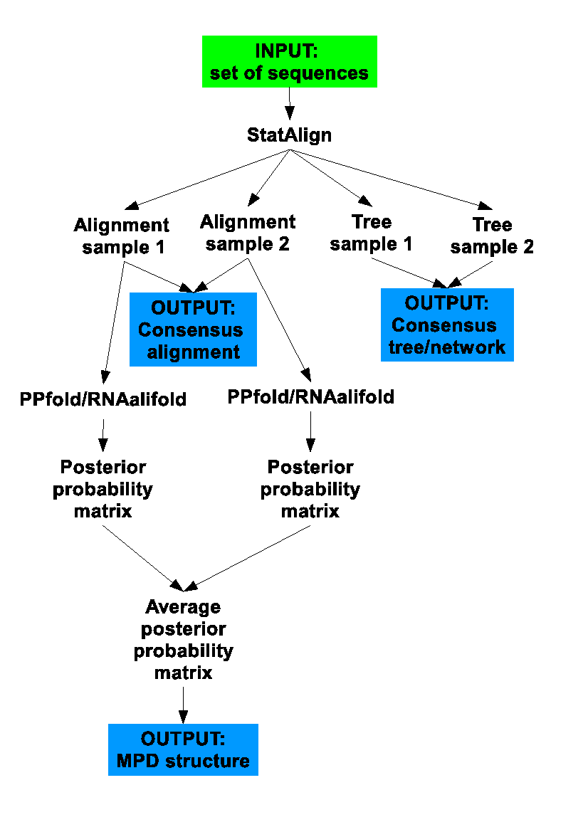
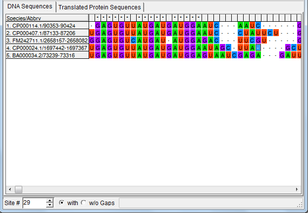
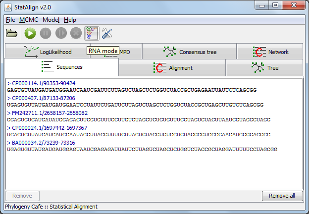
Before the RNA mode can be activated, a nucleotide alignment needs to be loaded. Once this is done the 'RNA mode' can activated by clicking on the 'RNA mode' icon below.
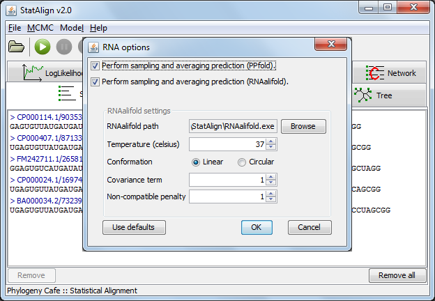
Activating the RNA mode brings up a settings dialog. Two different prediction methods are available for predicting structures from multiple alignment samples.
The first is an SCFG (Stochastic Context-Free Grammar) approach as implemented in PPfold ("Sampling and averaging (PPfold)").
Two predictions are produced using this approach: the standard sampling and averaging prediction, which produces a secondary structure from an averaged base-pairing probability matrix and a consensus evolutionary approach, which provides an information entropy value that takes into account contributions from alignment samples in addition to providing a secondary structure prediction.
A thermodynamic method ("Sampling and averaging (RNAalifold)")
can also be used, this method requires that user specify the RNAalifold executable (this shouldn't be necessary on Windows). This method allows the user to specify various
folding parameters such as the folding temperature and the genome conformation. The StatAlign GUI, however,
only provides some of these options. By running StatAlign from the command-line, additional RNAalifold parameters can be specified (see the RNAalifold manpage for a list of parameters).
Once the RNA mode is activated it will run alongside the normal StatAlign run.
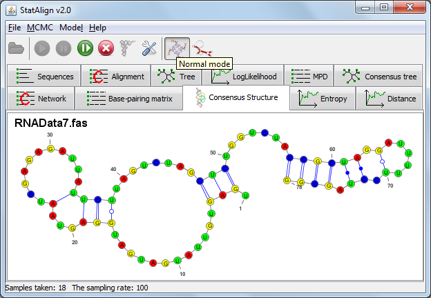
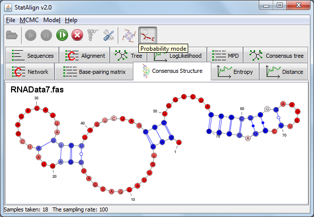
[ The RNA plugin ]During and after the run there are various tabs available for secondary structure visualisation. The first is the "Consensus Structure" tab which utilises VARNA (Darty et al. (2009)) to display the consensus secondary structure. Two modes are available: "Normal" mode which displays the nucleotides using a set of 4 colours to represent each base and a "Probability mode" which represents unpaired nucleotides in red and base-paired nucleotides in blue. Where the intensity of the red or blue represents the probability that a nucleotide is unpaired or the probability that a pair of nucleotides are base-paired, respectively.
Information entropy is a measure of the spread of a probability distribution. The PPfold method is a SCFG method (Stochastic Context-Free Grammar method)
used to predict secondary structures. This SCFG method places a probability distribution on secondary structures which means that the information entropy of this
probability distribution can be calculated (Anderson et. al. (2012), in preparation, available upon request).
A low entropy corresponds to a probability distribution where the probability mass is concentrated on
a few structures, whereas a high entropy indicates that the probability mass is spread over many structures - this is undesirable as it can be an
indication that there are many alternative secondary structures which are almost as equiprobable as the most probable structure.
The information entropy calculation provided in StatAlign has been extended to reflect that fact that the PPfold sampling and averaging method samples over
alignments, instead of using a single fixed alignment.
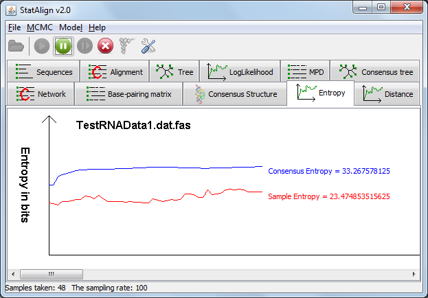
In the 'Entropy' tab, two line graphs are displayed depicting the 'Sample Entropy', which is the information entropy of the PPfold structure predictions
on individual alignment samples measured in bits, and 'Consensus Entropy' which is the extended information entropy that takes into account alignment space.
The 'Consensus Entropy' should approach a constant as the number of samples increases.
The final information entropy value can be found in the ".info" file on the header line corresponding to the consensus evolutionary prediction.
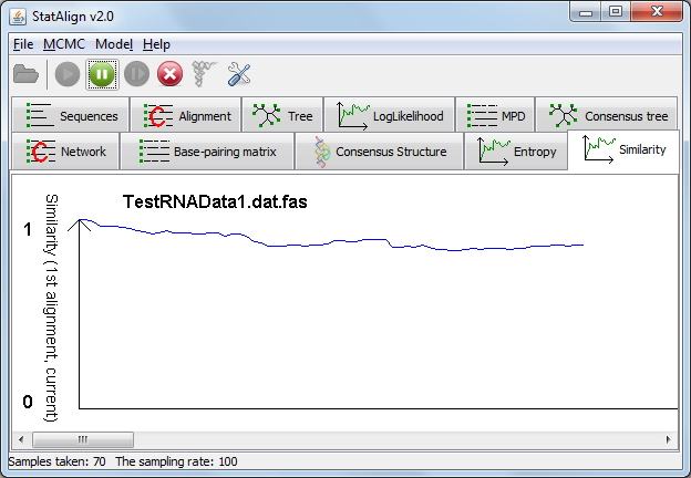
In the 'Similarity' tab, a graph is shown depicting the similarity between the first alignment sample and each of the subsequent alignment samples.
This provides a visual representation of auto-correlation between alignment samples. The similarity should gradually decrease and reach a plateau as the time between the first sample
and a given alignment becomes large, indicating that enough cycles have been taken between samples that they are no longer significantly auto-correlated.
Various secondary structure output files are available for each method in the StatAlign folder at the end of a run.
The naming convention used is: <dataset title>.<method>.<format extension>. The terms are defined as follows:
